Chapter 1
Using a Spreadsheet to Plot Curved Shapes - Part A
This topic is explored in the context of wanting to have a chart that, with a selectable reaction time assumption, would plot the distance in metres needed for an average sort of car to brake to a full stop over a range of speeds in km. per hour.
The two components of braking distance, that due to reaction time, and that
due to the speed, are also to be plotted.
A great many factors affect braking distance; the weight and size of the vehicle,
proceeding up hill down hill or on the flat, road surface conditions, tires
and more.
Reaction time can depend on such things as wakefulness and health.
To keep it simple, we assume that an average car with an average driver is proceeding
along a well-maintained dry flat straight highway enjoying good visibility.
A reasonable reaction time for our average driver will be taken to lie in the range
of 1 to 3 seconds.
Braking distance is proportional to the square of speed. This comes from the
study of mechanics, which finds that the energy of a moving body is proportional to
the square of its velocity. The degree of proportionality
is provided herein by a fixed multiplier of velocity squared.
When speed is given in kilometres per hour and stopping distance is desired
in metres, a suggested value for the multiplier is approximately 0.0059 for ordinary automobiles.
To begin, decide to employ the x-axis labels 10 through 160 in steps of 10 to represent
the speed. Decide also on an initial reaction time of 1.5 seconds.
Calculated values are usually created either in rows or in columns of cells. Because there
are only 255 columns in an Excel2000 sheet but there are 65,536 rows,
the
writer prefers to calculate values in columns to allow for a greater number
of values for each variable.
The following screen image shows the initial settings typed into the Excel cells.
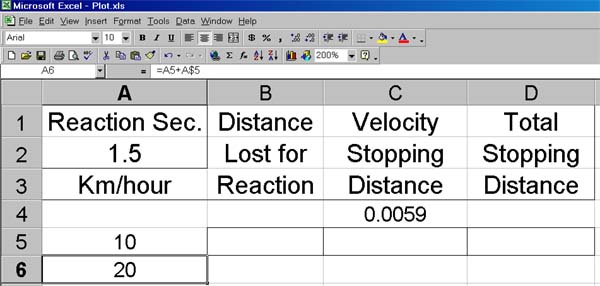
All cell entries are typed in as values except for that of A6.
A6 contains an expression that is seen on the
edit line, the row just above the
column headings. Mathematical expressions are always preceded by an "
="
symbol. The expression shows on the edit line because cell A6 has been
selected,
i.e., left clicked with the mouse. While selected, a cell is given a gray outline.
Cell A6 displays the value, (evaluated), of the expression. That value is 20 because cell
A5 in the expression has the value 10 as does A$5. As will
soon be explained, the difference between
cell address A5 and address A$5 becomes important when a copy of the contents of
cell A6 is pasted into another cell location.
To copy and paste, select a cell or cells, depress both
Ctrl and c (which puts a
copy on the "clipboard"), then move your mouse to another cell and select it. If
you then depress both
Ctrl and v, the copy will be made at the location of the newly
selected cell.
The next screen image shows the effect of copying A6 to A7.

A7 is selected and contains the expression A6 + A$5 versus the A5 +A$5 that A6 holds.
Copied cell addresses are normally relative but the $ sign before the row
address creates an absolute address when copies are made to any row in column A.
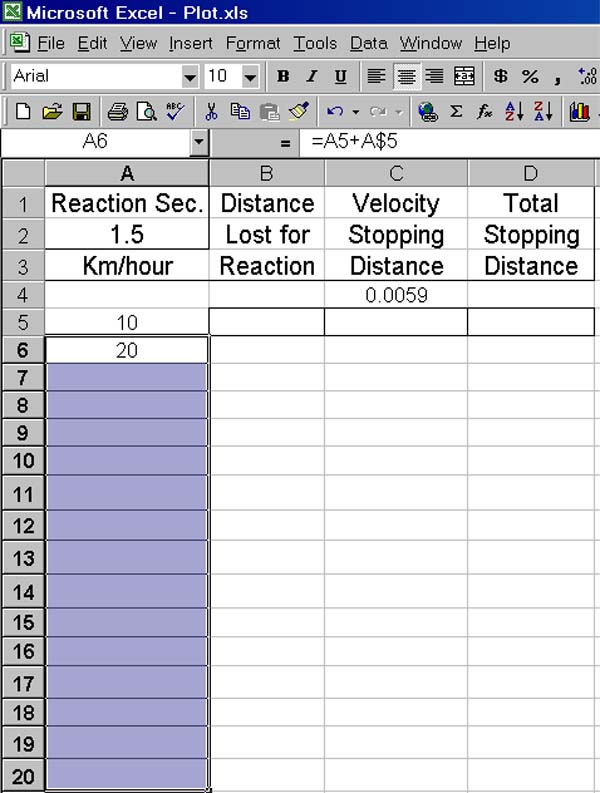
This makes it easy to create all the desired labels in one swoop. Just select
cell A6, depress
Ctrl and
c to put its content on the clipboard, place the
mouse on A7 as if to select it but now hold the left button down while sliding the cursor down column A to A20, release the button and a section of the column has been
selected as seen next.
(Note: As smaller images require less time to be transferred over the internet
than do larger images, subsequent screen prints will often be cropped to their more
essential portions. Also, when colour is unimportant, gray scale or even
black and white images will be employed.)
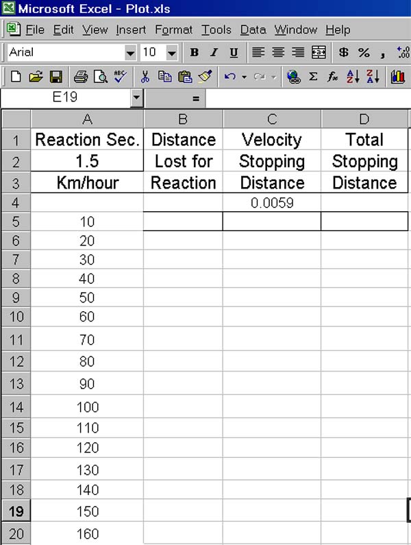
At this point, holding down Ctrl and left clicking v will populate A7 through A20 with
the desired labels as is seen next.
It is as easy as that and it gets easier. See the next screen image.
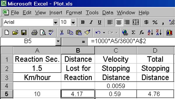
B5 has been selected and its typed contents are seen on the edit line. A5 is multiplied
by 1000 to convert from km to metres. The result is divided by 3600 to convert
from metres per hour to metres per second. That result is multiplied by the reaction
time in seconds to arrive at 4.17 metres of travel before brakes are applied.
Although not shown, the expression that was typed into cell C5 is "=A5^2*C$4", the
square of the speed multiplied by the given constant 0.0059. The result shown
in C5 is 0.59, the distance traveled between hitting the brakes and coming to a
full stop.
The expression typed into cell D5 is "=B5+C5" which forms the sum of the two distances
as the total distance traveled before coming to a full stop.
To populate cells B6 through D20 it is only necessary to select B5 through D5 as
a group, hold down
Ctrl and
c, and slide the cursor
down from B6 to B20, and then depress Ctrl
and v, for the result as is shown next.

The data is now available for plotting.
Next
Graphing of the calculated data is described in the next topic.