Chapter 4
Falling Bodies In a Fluid or Gas Part B - Numerical
solution of Differential Equations for Falling Bodies
A fundamental method for finding solutions to
non-linear
differential equations was provided by Vannevar Bush in:
The Differential Analyzer, V. Bush,
The Journal of the Franklin Institute, Vol.
212, No. 4, October 1931.
He began with a means for providing solutions to the linear
form of an equation and then modified the linear form by entering variable coefficients, v and g, using Input Tables. For each input table, an operator turned
a crank to keep an index on an applicable plotted curve as the solution proceeded.
For example, where gravity might previously be assumed to be constant through variations in height,
it could instead be input as some chosen function of height
by using an input table.
It is the Bush method, adapted for spreadsheet use, that is
employed herein for
finding solutions to non-linear differential equations.
For ease of discussion it will be assumed throughout this topic that falling bodies
start from rest and then increase in velocity as influenced by the acceleration
of gravity and an opposing drag force.
In the linear form the acceleration acting on the body will be g less some multiplier
of velocity.
The Linear Form
a = g - k * v = δv/δt (1)
This form is derived from Newton's second law, the force on the body F = m * a =
m * g
less a factor due to the resistance presented by the medium. That factor is termed
a drag force, Fd.
Dividing though by m, we find: a = g - Fd/
m.
Stokes found for a body moving slowly, creeping, in a viscous fluid that the drag
force could be taken as proportional to the velocity of the body.
As numerical methods are presumed, employ finite but small steps
of change that can be represented with symbols such as ∆, or D. We
then may write:
a = Dv/Dt
with the understanding that step size can be chosen small enough to meet the precision requirements
of an application.
Presume that one wishes to calculate the values that falling velocity, v,
and fallen distance, s, take on at successive small intervals in time, t, after a 1 kg body is dropped and that we know the values g ~= 10 metres per second and k =2.
Use a pen and paper for the calculations.
Decide to calculate at 1/10-second intervals. Divide the paper into 5 columns
headed in the first row by t, Dv, v, Ds, and s. To begin, populate the second
row with the initial values, all zeros. Next populate the remainder of the
first column with the successive values of the time t at which results are desired.
After fall has begun the body would normally arrive at the beginning of a calculation
step with a non- zero velocity. That velocity happens to be zero in the first step. The equation for acceleration, (1),
(g - k * v) = Dv/Dt
provides that:
Dv = Dt * (g - k * v). Then, for the first
step Dv = 1.0.
From here it is easy going. v is formed as the accumulation of the small steps
Dv. Each value of v in a step moves the body an incremental distance Ds = v * Dt.
Values of Ds are accumulated, negatively, to form s.
|
|
t |
Dv |
v |
Ds |
s |
|
|
|
0 |
0 |
0 |
0 |
0 |
|
|
|
0.1 |
1.0 |
1.0 |
0.1 |
-0.1 |
|
|
|
0.2 |
0.8 |
1.8 |
0.18 |
-0.28 |
|
For the next row and successive rows of calculation the procedure is unchanged.
The foregoing method of solving a differential equation using pen and paper is fundamentally
the same as was used by early astronomers to calculate planet orbits, planet masses
and planetary distances. Some of those calculations took a great many days.
Use a Spreadsheet
Today, although hand calculators have been used to relieve the tedium of pen and
paper calculation, the spreadsheet is better suited to the task. The spreadsheet
version, with graphs, is shown next.
Click the cell addresses following for their expressions.
Reynolds Number
There can be a question as to which model, Stokes or Lord
Rayleigh's, should be used for the drag force. The essential distinguishing feature
is whether the viscosity, μ, of the medium plays a role in the drag. Viscosity appears in the Reynold's number, R = p
* v * r /μ
, for a sphere,
(See Classical Mechanics, R. Douglas Gregory, Cambridge
University Press, 2006, pp83-85.) where r is the
radius of the sphere. The
reference concludes that the drag force is roughly proportional to v2 for 1,000 <
R < 100,000.
Since R is proportional to velocity, and in a case where there
is no initial velocity, one must conclude for a region near the very
beginning of fall in air, that the Stokes model applies. If the terminal velocity were
sufficiently high there would be a transitional period followed by a region in which the Rayleigh
model should be used.
The aforementioned reference provides values for the ratio μ/p for air, water, and castor
oil. The given values are: 1.5 * 10-5,
1.0 * 10-6,
and 1.04 * 10-3,
respectively.
Resistance Proportional to the Square of Velocity
In this case the equation for the acceleration of the body becomes:
a = g - k * v
2
= δv/δt
(2)
All that is needed to accommodate this form of the equation is to change the expression
in column D from =(D$3-F$3 *
E6) * (C7-C6) to =(D$3-F$3 *
E62)*(C7-C6)
for row 7 and
subsequent rows.
Calculated values will then change.
Is there a Source for Crosschecking?
This author has only located one other numerical solution
of this equation in the literature. That was in:
Euler's Method and Studies
of Motion, 11-12,Source Book for Programmable Calculators,
Texas Instruments Electronics
Series, McGraw-Hill, 1979. That solution was calculated at 1.0 second intervals
with g = 9.8 and k = 0.005 for a 1 Kg mass. Accordingly, Dt,
g and k were changed in the spreadsheet to these values. At t = 20 seconds, the Texas Instruments,
TI, velocity given was 44.27 m/s in good agreement with the value attained in the
spreadsheet, 44.2706. The fall distance found by TI was 760.594 m. That attained
in the spreadsheet was 781.511 m. No details of the TI algorithm were provided.
Clearly the algorithms are different in some way.
Exploration of the differences ascertained that full agreement with the 20 pairs
of values, (velocity, fall distance), given in the TI calculator reference could be
attained by halving the Dv contribution of the first step, i.e., changing (D$3-F$3 * E6
2)*(C7-C6)
to (D$3-F$3 * E6
2)
* (C7-C6)
/2 in row 7 only.
This then is the difference in the algorithms.
To determine a reasonable step size, trial calculations for the range 0 to
10 seconds were made with eight different step sizes Dt = 2, 1, 1/2, 1/4, 1/8, 1/16,
1/32, 1/64. Values attained on each trial for 0, 2, 4, 6, 8, and 10 seconds
were then plotted on the same graph to observe their convergence. These plots for
v and s are shown next.
Only the plots for the four or five largest step sizes appear to be distinguishable.
The fifth of these, 0.125, was chosen for the following wider range plot of v and
s. The 20 Texas Instruments pairs of values were superimposed for comparison.
Terminal Velocity
Return from the acceleration equation to the force equation. From the force equation:
m * a = m * g - k * v
2
The acceleration equation is: a = g - (k
* v2) / m.
Terminal velocity is reached
when g = (k * v
2) / m.
Thus
vt2
= (g * m)
/ k.
For the previous example, we used m=1, g = 9.8 and k = 0.005. For these values vt = 44.271887... metres
per second. The velocity attained at 30 seconds in the previous example was
44.2717799, a tiny bit short of vt.
A Different Formulation
Taking
Lord Rayleigh's approximation for the
drag force:
Fd = 1/2 *
ρ * A * Cd * v
2 .
Then using the force equation:
m * a = m * g - (1/2 *
ρ * A * Cd) *
v
2
or
a =
g - 1/2 *
1 / m *
ρ * A * Cd*
v
2
When
terminal velocity is reached:
2 * m * g =
ρ * A * Cd*
vt
2 or:
vt = [(2 * m * g) / (
ρ * A *
Cd)]
0.5.
Return to the acceleration
equation:
a = g - [1/2 *
ρ * A * Cd*
v
2] / m.
Substitute 2 *m *g / vt
2
for ρ * A
*
Cd to get:
a = g * [1 - v2/vt2],
an interesting
form of the equation. Of course it is no more than a rearrangement.
Under the approximation, the k seen in equation (2) is:
k = 1/2 * 1/m *
ρ*
A*
Cd
The Rayleigh approximation requires ρ the density
of the medium. For air near the earth's surface this is about 1.2 kg per cubic
metre. A is ~ the area that the body presents to the medium in its direction
of travel. Cd is a number describing
the smoothness or streamlining of the body.
Examples
The web-based, 1D, calculator given at the end of the next chapter and available
in the upper row
of tabs will be used to provide an example for a buoyant application.
As that calculator does not it self account for buoyancy, a method for causing its
results to include the effect of buoyancy is now given.
Buoyancy is an upward force due to the mass of the atmosphere that the object displaces.
The force equation for a buoyant object is:
F = m * g - m' * g - drag or
F= g * (m - m') - drag
Dividing the latter force equation through by m, the acceleration equation is then:
a = g * (1 - m' / m) - drag/m
Thus using g' = g * (1 - m' / m) rather than g
as input to the calculator will adjust the results to include the effect of buoyancy.
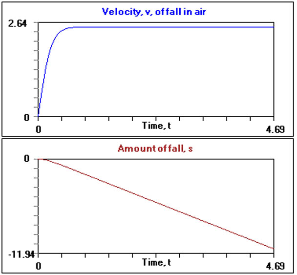
A latex spherical toy balloon inflated with air has a mass of about 0.0145 kg. Its radius is about 0.13 metres. Guess
Cd as 0.5. Call this the Light Balloon case. Plug these values into the calculator, using a step size of 0.01. Use g = 9.82, p = 1.2. Calculate the volume of the balloon as 4 / 3 * Pi * (0.13)^3 = 0.009203,
m' as 0.009203 * 1.2 = 0.01104 and then g' as 9.82
* (1 - 0.01104/.0145 = 2.343. The calculator's input data
is shown next:
Press Calculate, and the resulting charts are:
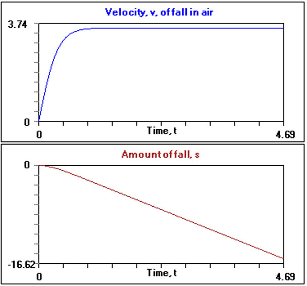
Tape a metal weight to the neck of the balloon such as a machine screw with washers
added to closely match the balloon's mass thus doubling its mass. Note that when
weighted, the balloon falls faster.
Plug this new value for m into the spreadsheet and employ a new value for g'.
(g' is recalculated as 6.082 if the mass has been doubled) The corresponding charts are shown next.
The light balloon appears to fall more slowly. Air resistance appears to slow the heavy balloon less
than it does the light balloon both for high and low velocities. But this
may not be the full story at the lower velocities. Recall that at very low
velocities we should use the Stokes model. Would that make any substantial
difference to the plotted results?
Use the 1D calculator to see how the falling rates of the two balloons compare when
the value for the density p of the atmosphere is reduced.
The story of Galileo finding that an iron ball and a same size wooden ball arrived
at the ground at the same when dropped together from the leaning tower is believed
by historians to be fiction. Nonetheless the story has inspired a great deal of
controversy over the years.
With very little additional research, and the links and material
provided in this topic, the viewer should be in a position to estimate the difference
in time of hitting the earth of Galileo's cannon and wooden balls.
Next
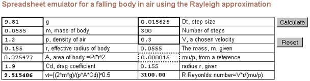
The next topic features a web-based calculator, an emulator of an interactive spreadsheet. It provides the viewer the opportunity to calculate
and plot solutions of the Lord Rayleigh form of the falling body differential equation. The viewer
may enter parameters and observe the results in a table and as plotted on charts. When buoyancy is a consideration, the user will need to calculate
and employ a g'.