Chapter 5
Spreadsheet Applied to Model the Kittinger Descent
The Kittinger Descent
Motivation
A motivation for constructing a spreadsheet that
included a representation of the standard atmosphere and took into account the variation
of gravitational attraction with altitude was a desire to model the 1960 descent
from a balloon of Captain Joseph Kittinger of the United States Air Force.
Briefly, his balloon reached an altitude of about 31,330 metres at the point when
he
exited his gondola. After about 12 seconds of fall, he opened a 1.8 metre stabilization
parachute and continued falling until his main parachute, 8.5 metres, deployed at
a height of about 5500 metres. He landed about eight minutes later.
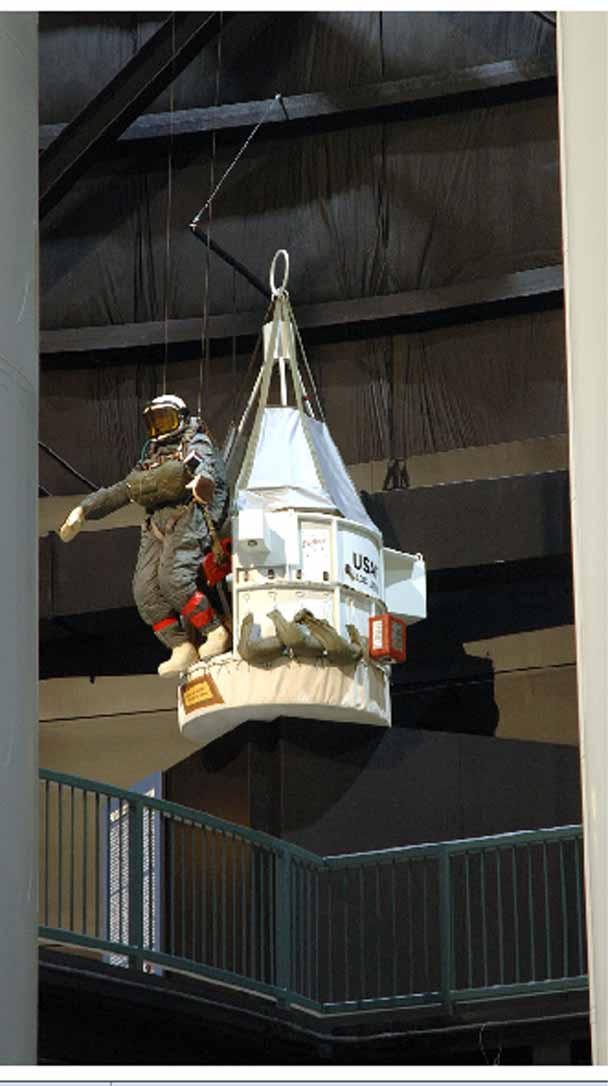
A picture of his gondola, below, taken at the Air Force Museum can be found
here.
Some Details
For details of the man, and of the records that were then set, see
here.
Two excerpts from the foregoing link follow:
1) Kittinger remained
at his peak altitude, over three times higher than a commercial airliner typically
flies, for about 12 minutes before he stepped off the "Highest Step in the World"
to begin his fall to the Earth's surface. In addition to his pressure suit, Kittinger
carried instruments and safety gear that weighed as much as he did. He also wore
several layers of clothing to help protect him against the extremes of his high-altitude
environment. During his fall, Kittinger experienced air temperatures as low as -94°F
(-70°C)!
2)
A final question to consider is why so many sources mistakenly claim that Joseph
Kittinger broke the sound barrier during his 1960 skydive. The most likely explanation
comes from the fact that these sources typically claim the maximum speed Kittinger
reached was 714 mph, just one digit off from the actual speed he attained of 614
mph. If Kittinger had reached the higher speed, he would have indeed been supersonic
and achieved approximately Mach 1.05. It seems probable that the author of some
official source accidentally miswrote the maximum speed and the mistake has been
replicated in numerous locations ever since.
Nevertheless,
the actual value of 614 mph comes from Joseph Kittinger himself in a 1960 article
he wrote for National Geographic and a subsequent book he authored describing the
jump. A direct quote from the former states:
"An hour and
thirty-one minutes after launch, my pressure altimeter halts at 103,300 feet. At
ground control the radar altimeters also have stopped-on readings of 102,800 feet,
the figure that we later agree upon as the more reliable. It is 7 o'clock in the
morning, and I have reached float altitude... Though my stabilization chute opens
at 96,000 feet, I accelerate for 6,000 feet more before hitting a peak of 614 miles
an hour, nine-tenths the speed of sound at my altitude."
What can be Taken from these Excerpts for Use in a Model?
The weight, or mass, of Kittinger and his equipment is not given. Excerpt 1) tells
us that the equipment weighed as much as he weighed. He was about 32 years
of age and likely quite fit. We will examine cases based on three possible weights
for Kittinger, 134, 154, and, 174 pounds. Doubling these weights to allow
for the equipment and converting to kilograms provides the approximate mass values
of 121.8, 140, and, 158.2 kg.
From Excerpt 2) it seems that the peak of his acceleration
was reached prior to reaching 90,000 feet of altitude. Measured by his altimeter?
Has he corrected, in this statement, for its offset from the ground radar altimeters?
Is his altimeter referenced to sea level or earth surface level?
Is the ground radar altimeter reading referenced to sea level or earth surface level?
What is his method of measuring velocity? Could the method be the rate of
change of his altimeter observations?
In order to Proceed with a Model of the Kittinger
Descent
We will presume that the ground radar altimeter reading is referenced to the local
earth surface. Converted to metres this will be ~ 31,333 metres. What
was the altitude of the radar set? We will use the altitude of Albuquerque
New Mexico, ~1509 metres. Thus the altitude of the balloon at the start of
the fall will be taken as ~ 32,842 metres above sea level.
We presume that he is referring to his altimeter with the statement "he
experienced no noticeable change in acceleration until he fell to 90,000 ft ".
We interpret this as relative to his initial
reading
of 103,300 ft. for the balloon height. Presuming the statement to be correct,
we can expect that maximum velocity was reached after dropping 4,054 metres from 32,842 metres,
that is, some time after falling to an altitude of 28,788 metres.
Objective of the Model:
We will attempt to model the fall to obtain the altitude at which he reached the peak velocity of 614 miles
per hour, 274.48 metres per second, and the time that was taken to reach that
peak velocity.
His stabilization chute had a radius of ~ 0.9 metres. This chute would be
expected to be only partly full until some time after maximum decent speed was reached.
The effective radius of the combination of chute and Kittinger must be found, as
must a value for the drag.
A density is also required for the combination of chute and man.
Reaching An Answer
The spreadsheet, using Exper = 2, that was introduced in Parts A and B of this
topic provides vertical velocity and the corresponding altitude and time.
We need to solve for values of the sphere radius, density
, and drag coefficient
given a maximum fall rate of 274.48 metres per second and three suggested
mass values.
This can be done by adding a steepest decent routine, introduced in Chapter 2, to
the spreadsheet. For those readers interested in adding the routine to the
downloadable spreadsheet it is seen next.
Although iteration to find the solutions is simple enough to be done "by hand" the
process is tedious. Moreover, a more capable steepest decent routine will
be employed in a later Topic and this application serves as an introduction to its
use.
The three solutions, one for each suggested mass value, 121.8, 140, and 158.2 kg
are seen next.
For all three solutions the low radius values seem more representative of Kittinger
and his equipment than of the chute. This suggests that the stabilization chute
is streaming out above Kittinger but not open to any significant extent. The most
significant drag may stem from Kittinger and his pack of instrumentation.
All three solutions show the time taken to reach the maximum fall rate of ~ 274.5
m/s as ~ 41 seconds at an altitude of about 25,778 metres.
Intuitively, this
answer does not seem to be far out of line. It is undoubtedly
not true in the
light of all the presumptions that that were needed and the unknown
precisions that
were involved.
A by-product of obtaining the three solutions was a range of possible drag coefficients,
1.49, 1.56, and 1.62 for the assemblage of a streaming chute, and Kittinger with
his equipment.
How well did the actual atmosphere over the New Mexico desert on August 16,
1960, correspond to the 1976 U.S. Standard Atmosphere? Although it is readily
conceivable that seasonal adjustments could be made to our atmospheric model, this has not been
attempted.
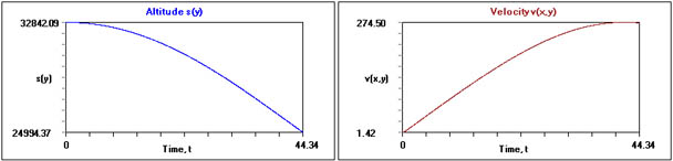
For interest, the web-based calculator linked in Chapter 6 and also found on the
upper row of tabs is used to provide graphs of altitude and velocity during the fall, to ~25,000 metres for the 140 kg case, seen
following:
Notwithstanding the uncertain parameters used in modeling the Kittinger decent,
the
spreadsheet, with its inclusion of a model of the standard atmosphere, should
be quite
useful
for estimating the behaviour of projectiles and falling bodies.
The Parameter Table
As has been mentioned, the macro varies some of the labels on the Par Sheet in accord
with the value, 0 through 4, of the Parameter Exper, which in this case has the
value 2 as is seen in the next table for modeling Kittinger's descent.
The ">", greater-than, character indicates that the value to its right is to
be provided by the user. These values show in bold type.
Three values, B4:B6, are permanent reminders of underlying assumptions.
The values B2 and B3 are calculated immediately when the platform altitude is entered
as possibly of interest to the user. Similarly, on entry of r in D2, D3:D4 and D6:D7
are calculated and on entry of d in D5, D6:D7 are immediately recalculated.
Some cell labels are applicable to other Experiments. Their associated values will remain blank. Some labels and their values are
common to all or most experiments.
The value for Target Altitude in D8 causes calculation to terminate when that altitude is reached.
Similarly calculation will terminate when the number of calculation steps given
in D10 is reached.
Notice the value 2.0 in B7 and 45 in B8. These are there to represent Kittinger's
little jump, up and out, to exit his gondola.
The Data Table
The first two rows of the data table are shown,
in two sections, following:
Row 0 shows the initial conditions.
Row 1 is special in that is the culmination of calculating eleven sub rows consisting
of: two rows calculated using 1/1024 of the
step size, followed by 9 rows each employing
twice the step size used in the previous step. This is equivalent to a whole
step at the specified step size.
The reason for doing this is that projectiles
may have a quite large initial velocity that drops quite quickly when an atmosphere
is encountered. The precision
of the calculation benefits from smaller step sizes in that initial
period of encountering the atmosphere
when deceleration is most rapid.
Data rows around the maximum fall rate are shown, in two sections, next:
One might note that the acceleration, Dv(y)/Dt, changes sign after the maximum fall
rate is reached,
Next
Chapter 6 will present applications of the spreadsheet
and calculator to non-pressurized and pressurized ballooning, high altitude research,
and ballistics, and will provide a link to the web-based version of this calculator.